MLB League Averages (ERA, BB, SO, BA) through the years

Diving into the Lahman Baseball Database, sometimes referred to as Baseball Databank

The first thing I want to do is see the total number of BB and SO per league each year. I have read in The Hidden Game ¹ that the number of walks exceeded strikeouts in the American League in the 1930s, and want to see it in the data. The MLB averages are on Baseball Reference but not separated by league. I am sure that data is somewhere on the web but I am going to find out myself.

Start with something easy. Get the number of ABs for the entire year. Using R. The data needed here is Batting.csv.

library(data.table)
library(dplyr)

batting <- data.table(read.csv("Batting.csv"))

batting |>
  group_by(yearID) |>
  summarise(AB = sum(AB)) |>
  arrange(desc(yearID))

It matches the data in Baseball Reference. Let’s add some statistics and separate by league.

batting |>
  filter(lgID == "AL") |>
  filter(yearID <= 1940 & yearID >= 1930) |>
  group_by(yearID) |>
  summarise(
    across(c(AB, BB, SO, H, G), sum),
    BA = sum(H) / sum(AB),
    BB_gt = ifelse(BB > SO, "BB greater than SO", "SO greater than BB")
  ) |>
  arrange(desc(yearID))

This shows up that indeed there were more walks than strikeouts for some years in the 1930s.

Now to see the per game statistics. To get number of games, use the Teams data because there is not an accurate measure of games using just the individual batting statistics.

teams <- data.table(read.csv("Teams.csv"))

al_games_year <- teams |>
  filter(lgID == 'AL') |>
  group_by(yearID) |>
  summarise(
    across(c(G), sum)
  )

batting |>
  filter(lgID == 'AL') |>
  filter(yearID <= 1940 & yearID >= 1930) |>
  group_by(yearID) |>
  summarise(
    across(c(AB, BB, SO, H, G), sum),
    BA = sum(H) / sum(AB),
    BB_gt = ifelse(BB > SO, "BB greater than SO", "SO greater than BB")
  ) |>
  inner_join(al_games_year, by = 'yearID') |>
  arrange(desc(yearID))
  
     yearID    AB    BB    SO     H   G.x    BA BB_gt                G.y
    <int> <int> <int> <int> <int> <int> <dbl> <chr>              <int>
 1   1940 43017  4494  4720 11674 13765 0.271 SO greater than BB  1238
 2   1939 42594  4654  4306 11866 13887 0.279 BB greater than SO  1230
 3   1938 42500  4924  4242 11935 13365 0.281 BB greater than SO  1226
 4   1937 43303  4776  4448 12178 13553 0.281 BB greater than SO  1244
 5   1936 43747  4853  4032 12657 13546 0.289 BB greater than SO  1236
 6   1935 42999  4550  3932 12033 13513 0.280 BB greater than SO  1222
 7   1934 42929  4608  4282 11966 13687 0.279 BB greater than SO  1230
 8   1933 42663  4365  3916 11637 13771 0.273 BB greater than SO  1216
 9   1932 43419  4408  4021 12015 13741 0.277 BB greater than SO  1230
10   1931 43683  4177  4032 12163 13837 0.278 BB greater than SO  1236
11   1930 42878  3963  4086 12337 13983 0.288 SO greater than BB  1232

See that the number of games in y (al_games_year) is much less than x (batting). Now to calculate per game statistics.

batting |>
  filter(lgID == 'AL') |>
  filter(yearID <= 1940 & yearID >= 1930) |>
  group_by(yearID) |>
  summarise(
    across(c(AB, BB, SO, H, G), sum),
    BA = sum(H) / sum(AB),
    BB_gt = ifelse(BB > SO, "BB greater than SO", "SO greater than BB")
  ) |>
  inner_join(al_games_year, by = 'yearID') |>
  mutate(BB_per_G = BB / G.y, SO_per_G = SO / G.y) |>
  select(yearID, G = G.y, AB, BB, SO, H, BA, BB_per_G, SO_per_G) |>
  arrange(desc(yearID))
  
     yearID     G    AB    BB    SO     H    BA BB_per_G SO_per_G
    <int> <int> <int> <int> <int> <int> <dbl>    <dbl>    <dbl>
 1   1940  1238 43017  4494  4720 11674 0.271     3.63     3.81
 2   1939  1230 42594  4654  4306 11866 0.279     3.78     3.50
 3   1938  1226 42500  4924  4242 11935 0.281     4.02     3.46
 4   1937  1244 43303  4776  4448 12178 0.281     3.84     3.58
 5   1936  1236 43747  4853  4032 12657 0.289     3.93     3.26
 6   1935  1222 42999  4550  3932 12033 0.280     3.72     3.22
 7   1934  1230 42929  4608  4282 11966 0.279     3.75     3.48
 8   1933  1216 42663  4365  3916 11637 0.273     3.59     3.22
 9   1932  1230 43419  4408  4021 12015 0.277     3.58     3.27
10   1931  1236 43683  4177  4032 12163 0.278     3.38     3.26
11   1930  1232 42878  3963  4086 12337 0.288     3.22     3.32

Now a basic line graph showing total walks and strikeouts per year.

grouped_BB_SS <- batting |>
  filter(lgID == 'AL') |>
  #filter(yearID <= 1940 & yearID >= 1930) |>
  group_by(yearID) |>
  summarise(
    across(c(AB, BB, SO, H, G), sum),
    BA = sum(H) / sum(AB),
    BB_gt = ifelse(BB > SO, "BB greater than SO", "SO greater than BB")
  ) |>
  inner_join(al_games_year, by = 'yearID') |>
  mutate(BB_per_G = BB / G.y, SO_per_G = SO / G.y) |>
  select(yearID, G = G.y, AB, BB, SO, H, BA, BB_per_G, SO_per_G) |>
  arrange(desc(yearID))

ggplot(grouped_BB_SS, aes(x = yearID)) +
  geom_line(aes(y = BB), color = "blue") +
  geom_line(aes(y = SO), color = "red") +
  labs(y = "BB or SO")

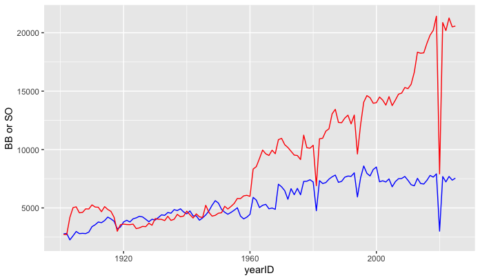
Above is a very quick line graph showing walks and strikeouts per year. The 1930s did have more walks (in blue) than strikeouts. I didn’t bother sprucing this graph up with a legend.

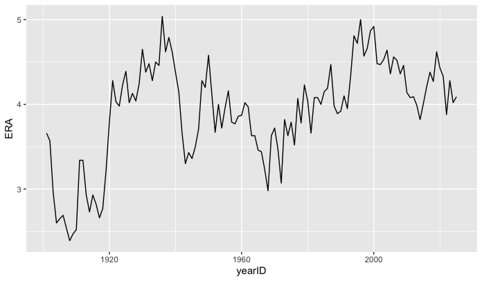
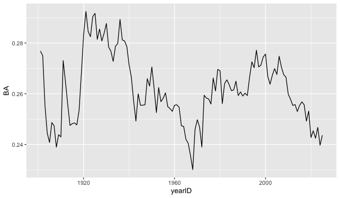
Below are quick graphs of American League ERA and BA per year as well

Thorn, John, and Palmer, Pete. The Hidden Game of Baseball. The University of Chicago Press, 2015, p. 144. ↩︎